TikZ
基础格式
%使用standalone格式
\documentclass[tikz,border=2pt]{standalone}
\begin{document}
\begin{tikzpicture}
\draw[step=1,color=gray!40] (-2,-2) grid (2,2);
\draw[->] (-3,0) -- (3,0);
\draw[->] (0,-3) -- (0,3);
\draw (0,0) circle (1);
\end{tikzpicture}
\end{document}
平移
% xshift ,x坐标轴平移。 yshift ,y坐标轴平移
% 注意xshift默认的单位并不是cm,如果要单位是cm需要写出来。
\begin{tikzpicture}
\draw[help lines] (0,0) grid (3,2);
\draw (0,0) -- (1,1);
\draw[red] (0,0) -- ([xshift=1cm] 1,1);
\end{tikzpicture}
旋转
% rotate旋转
\begin{tikzpicture}
\draw (0,0)[rotate=30]  ellipse (2 and 1);
\end{tikzpicture}
变量定义
\newcommand\XA{2}
\coordinate (A) at (\XA,\YA);
正方形
\tikzstyle{matrix}=[rectangle,thick,minimum size=1cm,draw=gray!80,fill=gray!20]
\node (m1) [matrix] at (0,0) [align=center] {};
矩形
\tikzstyle{matrix}=[rectangle,thick,minimum width=4mm,minimum height=3mm,draw=gray!80,fill=gray!20]
\node (m1) [matrix] at (0,0) [align=center] {};
平行四边形
\tikzstyle{matrix}=[trapezium,
thick,minimum width=8cm,
minimum height=6cm,
trapezium left angle=110,
trapezium right angle=70,
draw=gray!80,
fill=gray!20,
fill opacity=.8]
字体大小
\tiny
\small
\normalsize
\large
\Large
\LARGE
\huge

\node(SpatialTemporalFusion1) [SpatialTemporalFusion] at (\BA, -3.5) {\normalsize Spatial-Temporal Fusion};
圆
\tikzstyle{cell}=[circle,fill=black!25,minimum size=25pt,inner sep=0pt]
\node (n1) [node] at (0,0) [align=center] {$node_1$};
透明度
%fill opacity=.4, draw opacity=1
\documentclass[tikz]{standalone}
\begin{document}
\begin{tikzpicture}[thick,fill opacity=.4,draw opacity=1]
\draw[fill=yellow] (-9,-8) rectangle (9,8);
\draw[fill=red] (-9,-6) rectangle (2,6);
\draw[fill=orange,dashed] (-3,-5) rectangle (9,5);
\draw[fill=green,dotted] (-3,-4) rectangle (5,4);
\draw[fill=blue] (-6,-2) rectangle (0,2);
\end{tikzpicture}
\end{document}
箭头
\tikzstyle{arrow} = [->,>=stealth,draw=red!20,thick]

\draw [arrow] (n1) -- (n5);
% 线上添加文字
\draw [arrow] (n2) -- node[below]{$S_{1,2}$}(n1);
输出eps图
pdftops -eps <pdf file> <eps file>
去除pdf空白区域
pdfcrop <pdf file>
node换行(必须有align关键字)
\node at (-0.5,1)[draw, align=center]{example \\ example example};
波浪线
\documentclass{article} % say
\usepackage{tikz}
\usetikzlibrary{arrows,snakes,backgrounds}
\begin{document}
\begin{tikzpicture}
\draw [->,snake=snake] (0,0) -- (2,0);
\end{tikzpicture}
\end{document}
添加文本
\documentclass{article}
\usepackage{tikz}

\begin{document}

\begin{tikzpicture}
\node[draw] at (0,0) {some text};
\node[draw,align=left] at (3,0) {some text\\ spanning three lines\\ with manual line breaks};
\node[draw,text width=4cm] at (2,-2) {some text spanning three lines with automatic line breaks};
\end{tikzpicture}

\end{document}
tikzset
\documentclass{standalone}

\usepackage{tikz}
\begin{document}
\pagestyle{empty}

\def\layersep{2.5cm}

\tikzset{
  stations1/.pic ={
    \tikzstyle{arrow} = [->,>=stealth,draw=red!50,thick]
    \tikzstyle{arrow2} = [->,>=stealth,draw=red!80,thick]
    \tikzstyle{arrow3} = [->,>=stealth,draw=red,thick]
    \tikzstyle{node}=[circle,fill=black!25,minimum size=25pt,inner sep=0pt]
    %\tikzstyle{matrix}=[rectangle,thick,minimum size=1cm,draw=gray!80,fill=gray!20]
    %\tikzstyle{matrix}=[rectangle,thick,minimum width=8cm,minimum height=6cm,draw=gray!80,fill=gray!20,fill opacity=.8, align=right, text centered]
    \tikzstyle{matrix}=[rectangle,thick,minimum width=8cm,minimum height=6cm,draw=gray!80,fill=gray!20,fill opacity=.8]

    \node (m1) [matrix] at (0,0) [] {};
    \node (n1) [node] at (0,0) [align=center] {$node_1$};
    \node (n1) [node] at (0,0) [align=center] {$node_1$};
    \node (n2) [node] at (-6,0) [align=center] {$node_2$};
    \node (n3) [node] at (-5,5) [align=center] {$node_3$};
    \node (n4) [node] at (-5,-5) [align=center] {$node_4$};
    \node (n5) [node] at (0,-6) [align=center] {$node_5$};
    \node (n6) [node] at (6,-6) [align=center] {$node_6$};
    \node [draw,text width=4cm] at (4,6.5) {2021-1-16 12:00:00};

    \draw [arrow3] (n1) -- (n5);
    \draw [arrow3] (n1) -- (n6);
    \draw [arrow2] (n3) -- (n1);
    \draw [arrow3] (n2) -- (n1);
    \draw [arrow] (n2) -- (n4);
  },
}
\tikzset{
  stations2/.pic ={
  \tikzstyle{arrow} = [->,>=stealth,draw=red!50,thick]
  \tikzstyle{arrow2} = [->,>=stealth,draw=red!80,thick]
  \tikzstyle{arrow3} = [->,>=stealth,draw=red,thick]
  \tikzstyle{node}=[circle,fill=black!25,minimum size=25pt,inner sep=0pt]
  %\tikzstyle{matrix}=[rectangle,thick,minimum size=1cm,draw=gray!80,fill=gray!20]
  %\tikzstyle{matrix}=[rectangle,thick,minimum width=8cm,minimum height=6cm,draw=gray!80,fill=gray!20,fill opacity=.8, align=right, text centered]
  \tikzstyle{matrix}=[rectangle,thick,minimum width=8cm,minimum height=6cm,draw=gray!80,fill=gray!20,fill opacity=.8]

  \node (m1) [matrix] at (0,0) [] {};
  \node (n1) [node] at (0,0) [align=center] {$node_1$};
  \node (n1) [node] at (0,0) [align=center] {$node_1$};
  \node (n2) [node] at (-6,0) [align=center] {$node_2$};
  \node (n3) [node] at (-5,5) [align=center] {$node_3$};
  \node (n4) [node] at (-5,-5) [align=center] {$node_4$};
  \node (n5) [node] at (0,-6) [align=center] {$node_5$};
  \node (n6) [node] at (6,-6) [align=center] {$node_6$};
  \node [draw,text width=4cm] at (4,6.5) {2021-1-16 8:00:00};

  \draw [arrow3] (n1) -- (n5);
  \draw [arrow3] (n1) -- (n6);
  \draw [arrow2] (n3) -- (n1);
  \draw [arrow3] (n2) -- (n1);
  \draw [arrow] (n2) -- (n4);
  },
}

\tikzset{
  stations3/.pic ={
  \tikzstyle{arrow} = [->,>=stealth,draw=red!50,thick]
  \tikzstyle{arrow2} = [->,>=stealth,draw=red!80,thick]
  \tikzstyle{arrow3} = [->,>=stealth,draw=red,thick]
  \tikzstyle{node}=[circle,fill=black!25,minimum size=25pt,inner sep=0pt]
  %\tikzstyle{matrix}=[rectangle,thick,minimum size=1cm,draw=gray!80,fill=gray!20]
  %\tikzstyle{matrix}=[rectangle,thick,minimum width=8cm,minimum height=6cm,draw=gray!80,fill=gray!20,fill opacity=.8, align=right, text centered]
  \tikzstyle{matrix}=[rectangle,thick,minimum width=8cm,minimum height=6cm,draw=gray!80,fill=gray!20,fill opacity=.8]

  \node (m1) [matrix] at (0,0) [] {};
  \node (n1) [node] at (0,0) [align=center] {$node_1$};
  \node (n1) [node] at (0,0) [align=center] {$node_1$};
  \node (n2) [node] at (-6,0) [align=center] {$node_2$};
  \node (n3) [node] at (-5,5) [align=center] {$node_3$};
  \node (n4) [node] at (-5,-5) [align=center] {$node_4$};
  \node (n5) [node] at (0,-6) [align=center] {$node_5$};
  \node (n6) [node] at (6,-6) [align=center] {$node_6$};
  \node [draw,text width=4cm] at (4,6.5) {2021-1-16 04:00:00};

  \draw [arrow3] (n1) -- (n5);
  \draw [arrow3] (n1) -- (n6);
  \draw [arrow2] (n3) -- (n1);
  \draw [arrow3] (n2) -- (n1);
  \draw [arrow] (n2) -- (n4);
  },
}

\begin{tikzpicture}[scale=.4, font=\fontsize{12}{6}\selectfont]
    \pic[scale=.4] at (0,0) {stations1};
    \pic[scale=.4] at (2,-2) {stations2};
    \pic[scale=.4] at (4,-4) {stations3};

\end{tikzpicture}
% End of code
\end{document}
数学符号
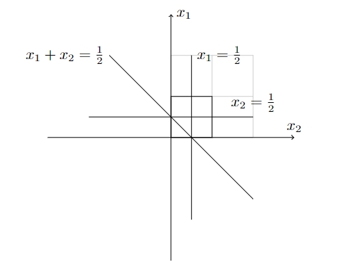
构建坐标系和添加函数
\begin{tikzpicture}
\draw[step=1,color=gray!40] (0,0) grid (2,2);
% 横坐标和纵坐标
\draw[->] (-3,0) -- (3,0) node[above] {$x_2$};
\draw[->] (0,-3) -- (0,3) node[right] {$x_1$};
\draw[draw=black] (0,0) rectangle (1, 1);
\draw[-] (2, -1.5) -- (-1.5,2) node[left,black] {$x_1+x_2=\frac{1}{2}$};
\draw[-] (-2, 0.5) -- (2,0.5) node[above,black] {$x_2=\frac{1}{2}$};
\draw[-] (0.5, -2) -- (0.5,2) node[right,black] {$x_1=\frac{1}{2}$};
\end{tikzpicture}

\end{document}
圆形
\draw (0,0) circle (1);
矩形
\draw[draw=black] (0,0) rectangle (1, 1);
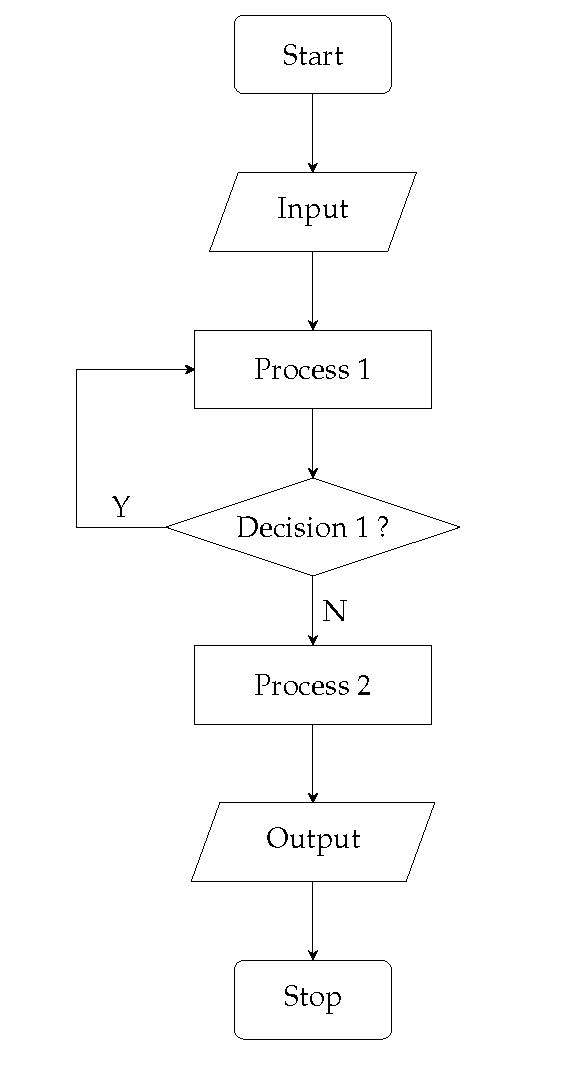
流程图
% texlive2015, pdflatex
\documentclass{article}
\usepackage{palatino}
\usepackage{tikz}
\usetikzlibrary{shapes.geometric, arrows}
\begin{document}
\thispagestyle{empty}
% 流程图定义基本形状
\tikzstyle{startstop} = [rectangle, rounded corners, minimum width = 2cm, minimum height=1cm,text centered, draw = black]
\tikzstyle{io} = [trapezium, trapezium left angle=70, trapezium right angle=110, minimum width=2cm, minimum height=1cm, text centered, draw=black]
\tikzstyle{process} = [rectangle, minimum width=3cm, minimum height=1cm, text centered, draw=black]
\tikzstyle{decision} = [diamond, aspect = 3, text centered, draw=black]
% 箭头形式
\tikzstyle{arrow} = [->,>=stealth]
\begin{tikzpicture}[node distance=2cm]
%定义流程图具体形状
\node[startstop](start){Start};
\node[io, below of = start, yshift = -1cm](in1){Input};
\node[process, below of = in1, yshift = -1cm](pro1){Process 1};
\node[decision, below of = pro1, yshift = -1cm](dec1){Decision 1 ?};
\node[process, below of = dec1, yshift = -1cm](pro2){Process 2};
\node[io, below of = pro2, yshift = -1cm](out1){Output};
\node[startstop, below of = out1, yshift = -1cm](stop){Stop};
\coordinate (point1) at (-3cm, -6cm);
%连接具体形状
\draw [arrow] (start) -- (in1);
\draw [arrow] (in1) -- (pro1);
\draw [arrow] (pro1) -- (dec1);
\draw (dec1) -- node [above] {Y} (point1);
\draw [arrow] (point1) |- (pro1);
\draw [arrow] (dec1) -- node [right] {N} (pro2);
\draw [arrow] (pro2) -- (out1);
\draw [arrow] (out1) -- (stop);
\end{tikzpicture}
\end{document}
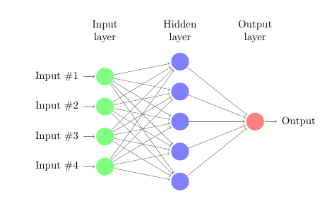
神经网络图
\documentclass{article}

\usepackage{tikz}
\begin{document}
\pagestyle{empty}

\def\layersep{2.5cm}

\begin{tikzpicture}[shorten >=1pt,->,draw=black!50, node distance=\layersep]
    \tikzstyle{every pin edge}=[<-,shorten <=1pt]
    \tikzstyle{neuron}=[circle,fill=black!25,minimum size=17pt,inner sep=0pt]
    \tikzstyle{input neuron}=[neuron, fill=green!50];
    \tikzstyle{output neuron}=[neuron, fill=red!50];
    \tikzstyle{hidden neuron}=[neuron, fill=blue!50];
    \tikzstyle{annot} = [text width=4em, text centered]

    % Draw the input layer nodes
    \foreach \name / \y in {1,...,4}
    % This is the same as writing \foreach \name / \y in {1/1,2/2,3/3,4/4}
        \node[input neuron, pin=left:Input \#\y] (I-\name) at (0,-\y) {};

    % Draw the hidden layer nodes
    \foreach \name / \y in {1,...,5}
        \path[yshift=0.5cm]
            node[hidden neuron] (H-\name) at (\layersep,-\y cm) {};

    % Draw the output layer node
    \node[output neuron,pin={[pin edge={->}]right:Output}, right of=H-3] (O) {};

    % Connect every node in the input layer with every node in the
    % hidden layer.
    \foreach \source in {1,...,4}
        \foreach \dest in {1,...,5}
            \path (I-\source) edge (H-\dest);

    % Connect every node in the hidden layer with the output layer
    \foreach \source in {1,...,5}
        \path (H-\source) edge (O);

    % Annotate the layers
    \node[annot,above of=H-1, node distance=1cm] (hl) {Hidden layer};
    \node[annot,left of=hl] {Input layer};
    \node[annot,right of=hl] {Output layer};
\end{tikzpicture}
% End of code
\end{document}
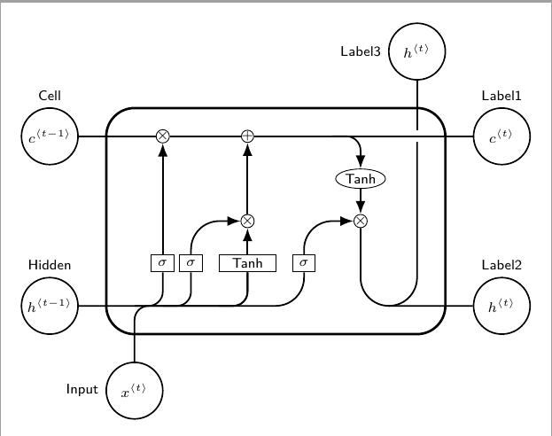
LSTM
\documentclass[tikz,border=10pt]{standalone}
\usepackage{tikz}
\usetikzlibrary{positioning, fit, arrows.meta, shapes}

\begin{document}

\begin{tikzpicture}[
    font=\sf \scriptsize,
    >=LaTeX,
    cell/.style={
        rectangle,
        rounded corners=5mm,
        draw,
        very thick,
        },
    operator/.style={
        circle,
        draw,
        inner sep=-0.5pt,
        minimum height =.2cm,
        },
    function/.style={
        ellipse,
        draw,
        inner sep=1pt
        },
    ct/.style={
        circle,
        draw,
        line width = .75pt,
        minimum width=1cm,
        inner sep=1pt,
        },
    gt/.style={
        rectangle,
        draw,
        minimum width=4mm,
        minimum height=3mm,
        inner sep=1pt
        },
    mylabel/.style={
        font=\scriptsize\sffamily
        },
    ArrowC1/.style={
        rounded corners=.25cm,
        thick,
        },
    ArrowC2/.style={
        rounded corners=.5cm,
        thick,
        },
    ]

%Start drawing the thing...
    % Draw the cell:
    \node [cell, minimum height =4cm, minimum width=6cm] at (0,0){};

    % Draw inputs named ibox#
    \node [gt] (ibox1) at (-2,-0.75) {$\sigma$};
    \node [gt] (ibox2) at (-1.5,-0.75) {$\sigma$};
    \node [gt, minimum width=1cm] (ibox3) at (-0.5,-0.75) {Tanh};
    \node [gt] (ibox4) at (0.5,-0.75) {$\sigma$};

   % Draw opérators   named mux# , add# and func#
    \node [operator] (mux1) at (-2,1.5) {$\times$};
    \node [operator] (add1) at (-0.5,1.5) {+};
    \node [operator] (mux2) at (-0.5,0) {$\times$};
    \node [operator] (mux3) at (1.5,0) {$\times$};
    \node [function] (func1) at (1.5,0.75) {Tanh};

    % Draw External inputs? named as basis c,h,x
    \node[ct, label={[mylabel]Cell}] (c) at (-4,1.5) {\empt{c}{t-1}};
    \node[ct, label={[mylabel]Hidden}] (h) at (-4,-1.5) {\empt{h}{t-1}};
    \node[ct, label={[mylabel]left:Input}] (x) at (-2.5,-3) {\empt{x}{t}};

    % Draw External outputs? named as basis c2,h2,x2
    \node[ct, label={[mylabel]Label1}] (c2) at (4,1.5) {\empt{c}{t}};
    \node[ct, label={[mylabel]Label2}] (h2) at (4,-1.5) {\empt{h}{t}};
    \node[ct, label={[mylabel]left:Label3}] (x2) at (2.5,3) {\empt{h}{t}};

% Start connecting all.
    %Intersections and displacements are used.
    % Drawing arrows
    \draw [ArrowC1] (c) -- (mux1) -- (add1) -- (c2);

    % Inputs
    \draw [ArrowC2] (h) -| (ibox4);
    \draw [ArrowC1] (h -| ibox1)++(-0.5,0) -| (ibox1);
    \draw [ArrowC1] (h -| ibox2)++(-0.5,0) -| (ibox2);
    \draw [ArrowC1] (h -| ibox3)++(-0.5,0) -| (ibox3);
    \draw [ArrowC1] (x) -- (x |- h)-| (ibox3);

    % Internal
    \draw [->, ArrowC2] (ibox1) -- (mux1);
    \draw [->, ArrowC2] (ibox2) |- (mux2);
    \draw [->, ArrowC2] (ibox3) -- (mux2);
    \draw [->, ArrowC2] (ibox4) |- (mux3);
    \draw [->, ArrowC2] (mux2) -- (add1);
    \draw [->, ArrowC1] (add1 -| func1)++(-0.5,0) -| (func1);
    \draw [->, ArrowC2] (func1) -- (mux3);

    %Outputs
    \draw [-, ArrowC2] (mux3) |- (h2);
    \draw (c2 -| x2) ++(0,-0.1) coordinate (i1);
    \draw [-, ArrowC2] (h2 -| x2)++(-0.5,0) -| (i1);
    \draw [-, ArrowC2] (i1)++(0,0.2) -- (x2);

\end{tikzpicture}
\end{document}
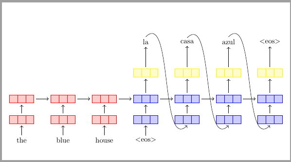
seq2seq
\documentclass[tikz,border=10pt]{standalone}
\usepackage{tikz}
\usetikzlibrary{positioning, fit, arrows.meta, shapes}


\begin{tikzpicture}[
    hid/.style 2 args={
      rectangle split,
      rectangle split horizontal,
      draw=#2,
      rectangle split parts=#1,
      fill=#2!20,
      outer sep=1mm}]
    % draw input nodes
    \foreach \i [count=\step from 1] in {the,blue,house,}
      \node (i\step) at (2*\step, -2) {\i};
    % draw output nodes
    \foreach \t [count=\step from 4] in {la,casa,azul,} {
      \node[align=center] (o\step) at (2*\step, +2.75) {\t};
    }
    % draw embedding and hidden layers for text input
    \foreach \step in {1,...,3} {
      \node[hid={3}{red}] (h\step) at (2*\step, 0) {};
      \node[hid={3}{red}] (e\step) at (2*\step, -1) {};
      \draw[->] (i\step.north) -> (e\step.south);
      \draw[->] (e\step.north) -> (h\step.south);
    }
    % draw embedding and hidden layers for label input
    \foreach \step in {4,...,7} {
      \node[hid={3}{yellow}] (s\step) at (2*\step, 1.25) {};
      \node[hid={3}{blue}] (h\step) at (2*\step, 0) {};
      \node[hid={3}{blue}] (e\step) at (2*\step, -1) {};
      \draw[->] (e\step.north) -> (h\step.south);
      \draw[->] (h\step.north) -> (s\step.south);
      \draw[->] (s\step.north) -> (o\step.south);
    }
    % edge case: draw edge for special input token
    \draw[->] (i4.north) -> (e4.south);
    % draw recurrent links
    \foreach \step in {1,...,6} {
      \pgfmathtruncatemacro{\next}{add(\step,1)}
      \draw[->] (h\step.east) -> (h\next.west);
    }
    % draw predicted-labels-as-inputs links
    \foreach \step in {4,...,6} {
      \pgfmathtruncatemacro{\next}{add(\step,1)}
      \path (o\step.north) edge[->,out=45,in=225] (e\next.south);
    }
  \end{tikzpicture}

  % End of code
\end{document}
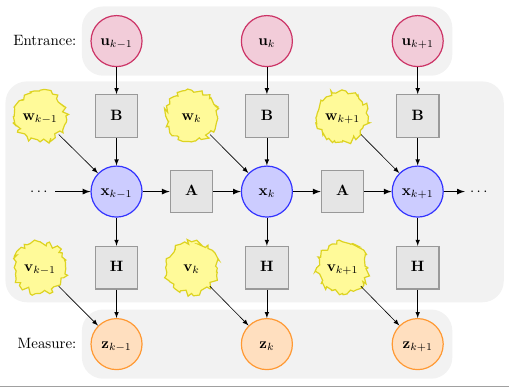
kalman-filter
\documentclass[a4paper,10pt]{article}

\usepackage[english]{babel}
\usepackage[T1]{fontenc}
\usepackage[ansinew]{inputenc}

\usepackage{lmodern}	% font definition
\usepackage{amsmath}	% math fonts
\usepackage{amsthm}
\usepackage{amsfonts}

\usepackage{tikz}

\usetikzlibrary{decorations.pathmorphing} % noisy shapes
\usetikzlibrary{fit}					% fitting shapes to coordinates
\usetikzlibrary{backgrounds}	% drawing the background after the foreground

\begin{document}

\begin{figure}[htbp]
\centering
% The state vector is represented by a blue circle.
% "minimum size" makes sure all circles have the same size
% independently of their contents.
\tikzstyle{state}=[circle,
                                    thick,
                                    minimum size=1.2cm,
                                    draw=blue!80,
                                    fill=blue!20]

% The measurement vector is represented by an orange circle.
\tikzstyle{measurement}=[circle,
                                                thick,
                                                minimum size=1.2cm,
                                                draw=orange!80,
                                                fill=orange!25]

% The control input vector is represented by a purple circle.
\tikzstyle{input}=[circle,
                                    thick,
                                    minimum size=1.2cm,
                                    draw=purple!80,
                                    fill=purple!20]

% The input, state transition, and measurement matrices
% are represented by gray squares.
% They have a smaller minimal size for aesthetic reasons.
\tikzstyle{matrx}=[rectangle,
                                    thick,
                                    minimum size=1cm,
                                    draw=gray!80,
                                    fill=gray!20]

% The system and measurement noise are represented by yellow
% circles with a "noisy" uneven circumference.
% This requires the TikZ library "decorations.pathmorphing".
\tikzstyle{noise}=[circle,
                                    thick,
                                    minimum size=1.2cm,
                                    draw=yellow!85!black,
                                    fill=yellow!40,
                                    decorate,
                                    decoration={random steps,
                                                            segment length=2pt,
                                                            amplitude=2pt}]

% Everything is drawn on underlying gray rectangles with
% rounded corners.
\tikzstyle{background}=[rectangle,
                                                fill=gray!10,
                                                inner sep=0.2cm,
                                                rounded corners=5mm]

\begin{tikzpicture}[>=latex,text height=1.5ex,text depth=0.25ex]
    % "text height" and "text depth" are required to vertically
    % align the labels with and without indices.

  % The various elements are conveniently placed using a matrix:
  \matrix[row sep=0.5cm,column sep=0.5cm] {
    % First line: Control input
    &
        \node (u_k-1) [input]{$\mathbf{u}_{k-1}$}; &
        &
        \node (u_k)   [input]{$\mathbf{u}_k$};     &
        &
        \node (u_k+1) [input]{$\mathbf{u}_{k+1}$}; &
        \\
        % Second line: System noise & input matrix
        \node (w_k-1) [noise] {$\mathbf{w}_{k-1}$}; &
        \node (B_k-1) [matrx] {$\mathbf{B}$};       &
        \node (w_k)   [noise] {$\mathbf{w}_k$};     &
        \node (B_k)   [matrx] {$\mathbf{B}$};       &
        \node (w_k+1) [noise] {$\mathbf{w}_{k+1}$}; &
        \node (B_k+1) [matrx] {$\mathbf{B}$};       &
        \\
        % Third line: State & state transition matrix
        \node (A_k-2)         {$\cdots$};           &
        \node (x_k-1) [state] {$\mathbf{x}_{k-1}$}; &
        \node (A_k-1) [matrx] {$\mathbf{A}$};       &
        \node (x_k)   [state] {$\mathbf{x}_k$};     &
        \node (A_k)   [matrx] {$\mathbf{A}$};       &
        \node (x_k+1) [state] {$\mathbf{x}_{k+1}$}; &
        \node (A_k+1)         {$\cdots$};           \\
        % Fourth line: Measurement noise & measurement matrix
        \node (v_k-1) [noise] {$\mathbf{v}_{k-1}$}; &
        \node (H_k-1) [matrx] {$\mathbf{H}$};       &
        \node (v_k)   [noise] {$\mathbf{v}_k$};     &
        \node (H_k)   [matrx] {$\mathbf{H}$};       &
        \node (v_k+1) [noise] {$\mathbf{v}_{k+1}$}; &
        \node (H_k+1) [matrx] {$\mathbf{H}$};       &
        \\
        % Fifth line: Measurement
        &
        \node (z_k-1) [measurement] {$\mathbf{z}_{k-1}$}; &
        &
        \node (z_k)   [measurement] {$\mathbf{z}_k$};     &
        &
        \node (z_k+1) [measurement] {$\mathbf{z}_{k+1}$}; &
        \\
    };

    % The diagram elements are now connected through arrows:
    \path[->]
        (A_k-2) edge[thick] (x_k-1)	% The main path between the
        (x_k-1) edge[thick] (A_k-1)	% states via the state
        (A_k-1) edge[thick] (x_k)		% transition matrices is
        (x_k)   edge[thick] (A_k)		% accentuated.
        (A_k)   edge[thick] (x_k+1)	% x -> A -> x -> A -> ...
        (x_k+1) edge[thick] (A_k+1)

        (x_k-1) edge (H_k-1)				% Output path x -> H -> z
        (H_k-1) edge (z_k-1)
        (x_k)   edge (H_k)
        (H_k)   edge (z_k)
        (x_k+1) edge (H_k+1)
        (H_k+1) edge (z_k+1)

        (v_k-1) edge (z_k-1)				% Output noise v -> z
        (v_k)   edge (z_k)
        (v_k+1) edge (z_k+1)

        (w_k-1) edge (x_k-1)				% System noise w -> x
        (w_k)   edge (x_k)
        (w_k+1) edge (x_k+1)

        (u_k-1) edge (B_k-1)				% Input path u -> B -> x
        (B_k-1) edge (x_k-1)
        (u_k)   edge (B_k)
        (B_k)   edge (x_k)
        (u_k+1) edge (B_k+1)
        (B_k+1) edge (x_k+1)
        ;

    % Now that the diagram has been drawn, background rectangles
    % can be fitted to its elements. This requires the TikZ
    % libraries "fit" and "background".
    % Control input and measurement are labeled. These labels have
    % not been translated to English as "Measurement" instead of
    % "Messung" would not look good due to it being too long a word.
    \begin{pgfonlayer}{background}
        \node [background,
                    fit=(u_k-1) (u_k+1),
                    label=left:Entrance:] {};
        \node [background,
                    fit=(w_k-1) (v_k-1) (A_k+1)] {};
        \node [background,
                    fit=(z_k-1) (z_k+1),
                    label=left:Measure:] {};
    \end{pgfonlayer}
\end{tikzpicture}

\caption{Kalman filter system model}
\end{figure}

\end{document}
重复元素
\documentclass{standalone}

\usepackage{tikz}
\begin{document}
\pagestyle{empty}

\def\layersep{10cm}

\tikzset{
  stations/.pic={
    \tikzstyle{arrow} = [->,>=stealth,draw=red!20,thick]
    \tikzstyle{arrow2} = [->,>=stealth,draw=red!50,thick]
    \tikzstyle{arrow3} = [->,>=stealth,draw=red,thick]
    \tikzstyle{node}=[circle,fill=black!25,minimum size=25pt,inner sep=0pt]

    \node (n1) [node] at (0,0) [align=center] {$node_1$};
    \node (n2) [node] at (-6,0) [align=center] {$node_2$};
    \node (n3) [node] at (-5,5) [align=center] {$node_3$};
    \node (n4) [node] at (-5,-5) [align=center] {$node_4$};
    \node (n5) [node] at (0,-6) [align=center] {$node_5$};
    \node (n6) [node] at (6,-6) [align=center] {$node_6$};

    \draw [arrow3] (n1) -- (n5);
    \draw [arrow3] (n1) -- (n6);
    \draw [arrow2] (n3) -- (n1);
    \draw [arrow3] (n2) -- (n1);
    \draw [arrow] (n2) -- (n4);
    },
}

\begin{tikzpicture}[scale=.4, font=\fontsize{12}{6}\selectfont]
    \pic[draw=blue] at (-1,1) {stations};
    \pic (stations) at (0,0) {stations};


\end{tikzpicture}
% End of code
\end{document}
时间序列
timeseries.dat
t x y z
1 2 3 7
2 1 2 8
3 0 0 8
4 2 0 10
5 3 0 11
6 2 -1 12
7 2 -1 12
8 2 -1 13
9 -1 -1 13
10 -2 -2 13
11 -4 -2 13
12 -4 -2 12
13 -5 -2 12
14 -5 -2 11
15 -5 -2 11
16 -6 -2 11
17 -6 -3 10
18 -6 -3 9
19 -5 -3 8
20 -5 -3 7
21 -5 -3 6
22 -4 -3 6
23 -2 -3 5
24 -2 -3 5
25 -2 -4 6
26 -1 -4 5
27 0 -3 5
28 1 -3 6
29 1 -3 6
30 1 -3 6
31 2 -3 7
32 2 -3 7
33 2 -3 7
34 2 -3 8
35 3 -2 8
36 2 -2 9
37 2 -3 10
38 3 -2 10
39 3 -2 11
40 1 -2 11
41 2 -2 11
42 2 -1 12
43 2 -1 12
44 2 -1 12
45 2 -1 12
46 1 -1 12
47 -1 -1 12
48 -1 -1 12
49 -1 -1 12
50 -2 -1 11
51 -3 -2 11
52 -3 -2 11
plot time dat
\documentclass{article}
\usepackage{pgfplots}
\pgfplotsset{compat=1.11}

\begin{document}
    \begin{tikzpicture}
        \begin{axis}[xlabel=time, ylabel=accel, legend pos=outer north east]
            \addplot[blue, mark=none] table[x=t, y=x] {timeseries.dat};
            \addlegendentry{x}
            \addplot[red, mark=none] table[x=t, y=y] {timeseries.dat};
            \addlegendentry{y}
            \addplot[green, mark=none] table[x=t,y=z] {timeseries.dat};
            \addlegendentry{z}
        \end{axis}
    \end{tikzpicture}
\end{document}
plot time_series
\documentclass{article}
\usepackage{pgfplots}
\pgfplotsset{compat=1.14}

\begin{document}
    \begin{tikzpicture}[scale=0.75]
        \begin{axis}[height=7cm, width=12cm, xlabel=Time, ylabel=DO, legend pos=outer north east, xtick={1, 2, 3, 4, 5, 6, 7, 8, 9},xticklabels={$T-5$, $T-4$, $T-3$, $T-2$, $T-1$, $T$, $T+1$, $T+2$, $T+3$}]
            % \addplot[color=blue, mark=square,] table[x=t, y=node1]{
            %     t node1
            %     1 2
            %     2 1
            %     3 0
            %     4 2
            %     5 3
            %     6 2
            %     7 4
            % };
            \addplot[color=blue, mark=square,] table[y=node1]{
                t node1
                1 2
                2 1
                3 0
                4 2
                5 3
                6 2
            };
            \addlegendentry{node1}
            \addplot[color=blue, mark=*, dashed] table[x=t, y=node1]{
                t node1
                6 2
                7 5
                8 6
                9 2
            };
            \addlegendentry{node1 prediction}
            \addplot[red, mark=square] table[x=t, y=node2]
            {
                t node2
                1 3
                2 2
                3 1
                4 4
                5 3
                6 5
            };
            \addlegendentry{node2}
            \addplot[color=green, mark=square,] table[x=t, y=node3]{
                t node3
                1 7
                2 8
                3 8
                4 9
                5 10
                6 8
            };
            \addlegendentry{node3}
        \end{axis}
    \end{tikzpicture}
\end{document}