pandas
数据读取
data read
# Reading a csv into Pandas.
df = pd.read_csv('uk_rain_2014.csv', encoding='utf-8', header=0)

# Read n rows
data = pd.read_csv('data.csv', nrows = 5)

# 转换为numpy
pd.DataFrame({"A": [1, 2], "B": [3, 4]}).to_numpy()

# Getting first x rows.
df.head(5)

# Getting last x rows.
df.tail(5)

# Changing column labels.
df.columns = ['water_year','rain_octsep', 'outflow_octsep','rain_decfeb', 'outflow_decfeb', 'rain_junaug', 'outflow_junaug']
df.head(5)

# Return a Numpy representation of the DataFrame.
df.values

# Finding out how many rows dataset has.
# 获取行数
len(df)
df.shape

# 获取列数
len(df.columns)

# Finding out basic statistical information on your dataset.
pd.options.display.float_format = '{:,.3f}'.format # Limit output to 3 decimal places.
df.describe()

# Constructing DataFrame from numpy ndarray:
df2 = pd.DataFrame(np.random.randint(low=0, high=10, size=(5, 5)),columns=['a', 'b', 'c', 'd', 'e'])

# Create dataframe创建DataFrame
df = pd.DataFrame(np.random.randn(8,5))

[{'points': 50, 'time': '5:00', 'year': 2010},
{'points': 25, 'time': '6:00', 'month': "february"},
{'points':90, 'time': '9:00', 'month': 'january'},
{'points_h1':20, 'month': 'june'}]
df = pd.DataFrame(ds)

# create dataframe
col_names =  ['A', 'B', 'C']
my_df  = pd.DataFrame(columns = col_names)

# create from numpy
pd.DataFrame(np_array)

# Iterate Over Columns in Pandas Dataframe
# 迭代列名和列
for (colname,colval) in df.iteritems():
    print(colname, colval.values)

# enumerate() to Iterate Over Columns Pandas
# 迭代列序号和列数据
for (index, colname) in enumerate(df):
    print(index, df[colname].values)

# 多个索引筛选MultiIndex
df[df.index.get_level_values(0) == 1]

# 重置多索引(两个索引)
df = df.reset_index(level=[0,1])
insert插入
# append 插入一行(已经被废弃)
df.append(df2, ignore_index=True)

# 连续插入一行
lst = []

for new_row in items_generation_logic:
   lst.append(new_row)

# create extension
df_extended = pd.DataFrame(lst, columns=['A', 'B', 'C'])
# or columns=df.columns if identical columns

# concatenate to original
out = pd.concat([df, df_extended])

# 插入列, 插入第一列
df.insert(0,'date',date)

# 默认插入到第一列
df['date']=date

# 连续插入一行
df.loc[-1] = [2, 3, 4]  # adding a row
df.index = df.index + 1  # shifting index
df = df.sort_index()  # sorting by index
数据透视表
数据分析中经常需要进行“行列转化”。pandas.melt()函数可以实现将 “宽数据” → “长数据”的一种列转行变换。类似于Excel中的透视表pivot和逆透视表的操作。
# 构建测试数据集
import pandas as pd
df = pd.DataFrame({'A': {0: 'a', 1: 'b', 2: 'c'},
                   'B': {0: 1, 1: 3, 2: 5},
                   'C': {0: 2, 1: 4, 2: 6}
                   })
df
'''
   A  B  C
0  a  1  2
1  b  3  4
2  c  5  6
'''

# 默认转换
pd.melt(df, id_vars=['A'], value_vars=['B'])
'''
   A variable  value
0  a        B      1
1  b        B      3
2  c        B      5
'''

pd.melt(df, id_vars=['A'], value_vars=['B', 'C'])
'''
   A variable  value
0  a        B      1
1  b        B      3
2  c        B      5
3  a        C      2
4  b        C      4
5  c        C      6
'''
数据处理
get data from column & row 数据过滤
# Getting a column by label
# 获取列数据
df['rain_octsep']

# 获得多列
df[['a', 'b']]

# Getting a column by label using .
df.rain_octsep

# Creating a series of booleans based on a conditional
df.rain_octsep < 1000 # Or df['rain_octsep] < 1000

# Using a series of booleans to filter
# 数据筛选
df[df.rain_octsep < 1000]

# convert pandas float series to int and filter
# 数据转换
df = df[df['hour'].astype(int)==0]

# 类型转换
df['timestamp'] = df['datetime'].astype(int)

# 多重数据过滤
df[['algo_name', 'rmse']][(df['nout']==2) & (df['dataset']=='beijing_do_s') & (df['filter'].isna())].sort_values(by='rmse')

# 过滤值是NaN的行
df['filter'].isna()

# 过滤NaN的行
df['filter'].notna()

# 正则表达式
df[df['name'].str.contains(r'\d{6,}')]

# line replaces None with NaN
# 替换Nan值为None
df['column'].replace('None', np.nan, inplace=True)

# Filtering by multiple conditionals(Can't use the keyword 'and')
# 多条件过滤
df[(df.rain_octsep < 1000) & (df.outflow_octsep < 4000)]

# Filtering by string methods
df[df.water_year.str.startswith('199')]

# loc gets rows (or columns) with particular labels from the index.
# iloc gets rows (or columns) at particular positions in the index (so it only takes integers).
# ix usually tries to behave like loc but falls back to behaving like iloc if a label is not present in the index.

# Getting a row via a label-based index, 'Andrade' is the index of last_name
df.loc['Andrade']

# Select columns with .loc using the names of the columns
df.loc[['Andrade', 'Veness'], ['first_name', 'address', 'city']]

# To select rows whose column value equals a scalar
df.loc[df['column_name'] == some_value]

# To select rows whose column value does not equal some_value
df.loc[df['column_name'] != some_value]

# If you have multiple values you want to include, put them in a list (or more generally, any iterable) and use isin
df.loc[df['column_name'].isin(['one','three'])]

# Combine multiple conditions with &
df.loc[(df['column_name'] == some_value) & df['other_column'].isin(some_values)]

# isin returns a boolean Series, so to select rows whose value is not in some_values
df.loc[~df['column_name'].isin(some_values)]

# Getting a row via a numerical index
# 根据索引获取行
df.iloc[30]

# Getting a columnes
df.iloc[:, 0]

# Getting a row via a label-based or numerical index
df.ix['1999/00'] # Label based with numerical index fallback *Not recommended

# Setting a new index from an existing column
# 设置索引
df = df.set_index(['water_year'])
df.head(5)

# Returning an index to data
df = df.reset_index('water_year')
df.head(5)

# remove all duplicates and keep one 去重
df.drop_duplicates()

# 去除重复行
df = pd.DataFrame({"A":["foo", "foo", "foo", "bar"], "B":[0,1,1,1], "C":["A","A","B","A"]})

     A  B  C
0  foo  0  A
1  foo  1  A
2  foo  1  B
3  bar  1  A

df.drop_duplicates(subset=['A', 'C'], keep='last')

     A  B  C
1  foo  1  A
2  foo  1  B
3  bar  1  A

# reset index
df = df.reset_index(drop=True)

# or statement
new_df[(new_df['hour'].astype(int)==0) | (new_df['hour'].astype(int)==8) | (new_df['hour'].astype(int)==16)]

# loop iterate over rows in a DataFrame
for index, row in df.iterrows():
    print(row['dateTime'], row['CODMn'])

# tolist
# 转换为列表
List = df['row1'].tolist()

# get_loc
unique_index = pd.Index(list('abc'))
# 1
unique_index.get_loc('b')

# 获取列名
# iterating the columns
for col in data.columns:
    print(col)
lambda
df = pd.DataFrame([[1, 2.12], [3.356, 4.567]])
df.map(lambda x: len(str(x)))

# 忽略nan
df_copy = df.copy()
df_copy.iloc[0, 0] = pd.NA
df_copy.map(lambda x: len(str(x)), na_action="ignore")
平均划分20份
df = np.array_split(df, 20)
区间范围划分bins
data = pd.Series([1, 2, 3, 4, 5, 6, 7, 8, 9, 10])

# 将数据划分为三个频率区间(分箱操作)(bins)
bins = 3
result = pd.cut(data, bins=bins, labels=[f'区间{i+1}' for i in range(bins)])
计算差分的频率
result_count = pd.cut(allcom_df['factor'], bins=bins).value_counts()
diff 差分
df = pd.DataFrame({'a': [1, 2, 3, 4, 5, 6],
                   'b': [1, 1, 2, 3, 5, 8],
                   'c': [1, 4, 9, 16, 25, 36]})
df
   a  b   c
0  1  1   1
1  2  1   4
2  3  2   9
3  4  3  16
4  5  5  25
5  6  8  36

df.diff()
     a    b     c
0  NaN  NaN   NaN
1  1.0  0.0   3.0
2  1.0  1.0   5.0
3  1.0  1.0   7.0
4  1.0  2.0   9.0
5  1.0  3.0  11.0
滑动窗口rolling
df = pd.DataFrame({'B': [0, 1, 2, np.nan, 4]})
df
     B
0  0.0
1  1.0
2  2.0
3  NaN
4  4.0

df.rolling(2).sum()
     B
0  NaN
1  1.0
2  3.0
3  NaN
4  NaN
排序
# 指定列名 & 指定行属性 & 按值排序
df[['algo_name', 'nout', 'rmse']][(df['nout']==1) & (df['dataset']=='beijing_do')].sort_values(by='algo_name')

# 根据某一列排序
df.sort_index(axis=1)

# 根据某一行进行排序
df.sort_index()

# 根据某一列值进行排序
df.sort_values(by='a')

# 根据某列排序,并重置index
df2 = df.sort_values(by=['x','y'],ignore_index=True)

s = pd.Series([np.nan, 1, 3, 10, 5])
# series 升序
s.sort_values(ascending=True)
# series 降序
s.sort_values(ascending=False)
修改数据
#修改index为‘1’,column为‘name’的那一个值为aa
df.loc[1,'name'] = 'aa'

#修改index为‘1’的那一行的所有值。
df.loc[1] = ['bb','ff',11]

#修改index为‘1’,column为‘name’的那一个值为bb,age列的值为11。
df.loc[1,['name','age']] = ['bb',11]

#iloc[row_index, column_index]
#修改某一无素
df.iloc[1,2] = 19

##修改一整列
df.iloc[:,2] = [11,22,33]

#修改一整行
df.iloc[0,:] = ['lily','F',15]

#根据条件修改
df.loc[df1['stream'] == 2, ['feat','another_feat']] = 'aaaa'
print df
   stream        feat another_feat
a       1  some_value   some_value
b       2        aaaa         aaaa
c       2        aaaa         aaaa
d       3  some_value   some_value
Add default values
#replace nan with an empty string or some other default value.
data.country = data.country.fillna('')

#a calculation like taking the mean duration can help us even the dataset out. It’s not a great measure, but it’s an estimate of what the duration could be based on the other data.
data.duration = data.duration.fillna(data.duration.mean())
move column
a
#   x1  x2
#0   0   5
#1   1   6
#2   2   7
#3   3   8
#4   4   9

a.x2 = a.x2.shift(1)
#   x1  x2
#0   0 NaN
#1   1   5
#2   2   6
#3   3   7
#4   4   8
Remove rows & columns
#Drop columns
df.drop(['B', 'C'], axis=1)
df.drop(columns=['B', 'C'])

#Drop a row by index
df.drop([0, 1])

#Dropping all rows with any NA values is easy:
data.dropna()

# 去除inf和nan
df.replace([np.inf, -np.inf], np.nan).dropna(axis=1)

#we can also drop rows that have all NA value
data.dropna(how=’all’)

#We can also put a limitation on how many non-null values need to be in a row in order to keep it (in this example, the data needs to have at least 5 non-null values):
data.dropna(thresh=5)

#Let’s say for instance that we don’t want to include any movie that doesn’t have information on when the movie came out:
data.dropna(subset=[‘title_year’])

#update data with drop nan
data = data.dropna(subset=[water_column])

#Drop the columns with that are all NA values:
data.dropna(axis=1, how=’all’)

#Drop all columns with any NA values:
data.dropna(axis=1, how=’any’)
判断数据
# 判断是否存在nan值,如果存在返回True
df['col_name'].isnull().values.any()
apply function
# Applying a function to a column
def base_year(year):
    base_year = year[:4]
    base_year= pd.to_datetime(base_year).year
    return base_year

df['year'] = df.water_year.apply(base_year)
df.head(5)
groupby
# Manipulating structure (groupby, unstack, pivot)
# Grouby
df.groupby(df.year // 10 *10).max()

decade_rain = df.groupby([df.year // 10 * 10, df.rain_octsep // 1000 * 1000])[['outflow_octsep','outflow_decfeb','outflow_junaug']].mean()
decade_rain

# View Groups
ipl_data = {'Team': ['Riders', 'Riders', 'Devils', 'Devils', 'Kings',
         'kings', 'Kings', 'Kings', 'Riders', 'Royals', 'Royals', 'Riders'],
         'Rank': [1, 2, 2, 3, 3,4 ,1 ,1,2 , 4,1,2],
         'Year': [2014,2015,2014,2015,2014,2015,2016,2017,2016,2014,2015,2017],
         'Points':[876,789,863,673,741,812,756,788,694,701,804,690]}
df = pd.DataFrame(ipl_data)

print df.groupby('Team').groups

{'Kings': Int64Index([4, 6, 7],      dtype='int64'),
'Devils': Int64Index([2, 3],         dtype='int64'),
'Riders': Int64Index([0, 1, 8, 11],  dtype='int64'),
'Royals': Int64Index([9, 10],        dtype='int64'),
'kings' : Int64Index([5],            dtype='int64')}

# multiple columns
print df.groupby(['Team','Year']).groups

#('Kings', 2014): Int64Index([4], dtype='int64'),
#('Royals', 2014): Int64Index([9], dtype='int64'),
#('Riders', 2014): Int64Index([0], dtype='int64'),
#('Riders', 2015): Int64Index([1], dtype='int64'),
#('Kings', 2016): Int64Index([6], dtype='int64'),
#('Riders', 2016): Int64Index([8], dtype='int64'),
#('Riders', 2017): Int64Index([11], dtype='int64'),
#('Devils', 2014): Int64Index([2], dtype='int64'),
#('Devils', 2015): Int64Index([3], dtype='int64'),
#('kings', 2015): Int64Index([5], dtype='int64'),
#('Royals', 2015): Int64Index([10], dtype='int64'),

# Iterating through Groups
grouped = df.groupby('Year')

for name,group in grouped:
    print name
    print group

2014
   Points  Rank     Team   Year
0     876     1   Riders   2014
2     863     2   Devils   2014
4     741     3   Kings    2014
9     701     4   Royals   2014

2015
   Points  Rank     Team   Year
1     789     2   Riders   2015
3     673     3   Devils   2015
5     812     4    kings   2015
10    804     1   Royals   2015

2016
   Points  Rank     Team   Year
6     756     1    Kings   2016
8     694     2   Riders   2016

2017
   Points  Rank    Team   Year
7     788     1   Kings   2017
11    690     2  Riders   2017

# Select a Group
grouped = df.groupby('Year')
print grouped.get_group(2014)

   Points  Rank     Team    Year
0     876     1   Riders    2014
2     863     2   Devils    2014
4     741     3   Kings     2014
9     701     4   Royals    2014

# Aggregations
grouped = df.groupby('Year')
print(grouped['Points'].agg(np.mean))

Year
2014   795.25
2015   769.50
2016   725.00
2017   739.00
Name: Points, dtype: float64


# 合并多个行
# Group by TradingTime and aggregate BuyOrderQueue and SellOrderQueue
grouped = orderqueue_df.groupby('TradingTime').agg({
   'BuyOrderQueue': lambda x: [item for item in x if isinstance(item, list)],
   'SellOrderQueue': lambda x: [item for item in x if isinstance(item, list)]
})

grouped['BuyOrderQueue'] = grouped['BuyOrderQueue'].apply(lambda x: x[0] if x else [])
grouped['SellOrderQueue'] = grouped['SellOrderQueue'].apply(lambda x: x[0] if x else [])
COMBINING DATASETS合并数据
rain_jpn = pd.read_csv('notebook_playground/data/jpn_rain.csv')
rain_jpn.columns = ['year', 'jpn_rainfall']

uk_jpn_rain = df.merge(rain_jpn, on='year')
uk_jpn_rain.head(5)

# pd.merge
result = pd.merge(user_usage, user_device[['use_id', 'platform', 'device']], on='use_id')
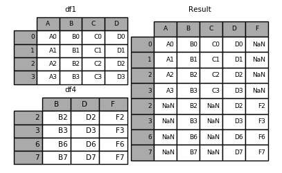
append & concat
result = pd.concat(frames)
result = df1.append(df4, ignore_index=True)
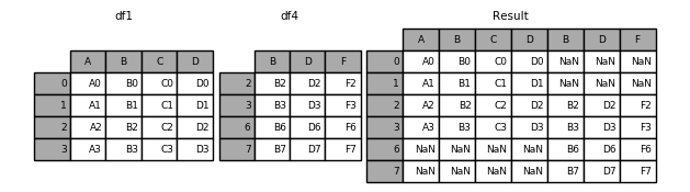
concat
result = pd.concat([df1, df4], axis=1, sort=False)
SAVING YOUR DATASETS数据保存
# Saving your data to a csv
df.to_csv('uk_rain.csv',index=False)
时间序列time series
时间日期处理datetime
# 字符串转换为date
pd.to_datetime(base_df['dateTime'],format='%d%b%Y:%H:%M:%S.%f')s


# selecting DataFrame rows between two dates
start = datetime.datetime(2014,4,2)
end = datetime.datetime(2017,12,15,4)
base_df['dateTime'] = pd.to_datetime(base_df['dateTime'])
base_df = base_df.set_index(['dateTime'])
new_df = base_df.loc[start:end]
# or
df = pd.DataFrame(np.random.random((200,3)))
df['date'] = pd.date_range('2000-1-1', periods=200, freq='D')
mask = (df['date'] > '2000-6-1') & (df['date'] <= '2000-6-10')
print(df.loc[mask])
# or
df = df[(df['date'] > '2000-6-1') & (df['date'] <= '2000-6-10')]

# 转换成时间戳
cod_df['datetime'] = pd.to_datetime(cod_df["datetime"]).astype(int)/10**9

# 时间序列整理datetime format
df = pd.DataFrame({"Date": ["26-12-2007", "27-12-2007", "28-12-2007"]})
df["Date"] = pd.to_datetime(df["Date"]).dt.strftime('%Y-%m-%d')
df["Date"] = pd.to_datetime(df["Date"]).dt.strftime('%Y-%m-%d %H:%M:%S')

# 时间范围生成range
DatetimeIndex(['2018-01-01 00:00:00', '2018-01-01 01:00:00',
               '2018-01-01 02:00:00'],
              dtype='datetime64[ns]', freq='H')
dti = pd.date_range('2018-01-01', periods=3, freq='H')

DatetimeIndex(['2018-04-24 00:00:00', '2018-04-25 12:00:00',
               '2018-04-27 00:00:00'],
              dtype='datetime64[ns]', freq=None)
pd.date_range(start='2018-04-24', end='2018-04-27', periods=3)


# Timedelta
# Timedelta('1 days 02:00:00')
ts = pd.Timestamp('2016-10-30 00:00:00', tz='Europe/Helsinki')

# Respects absolute time
# Timestamp('2016-10-30 23:00:00+0200', tz='Europe/Helsinki')
ts + pd.Timedelta(days=1)
# Respects calendar time
# Timestamp('2016-10-31 00:00:00+0200', tz='Europe/Helsinki')
ts + pd.DateOffset(days=1)

           A      B          C
# 0 2018-01-01 0 days 2018-01-01
# 1 2018-01-02 1 days 2018-01-03
# 2 2018-01-03 2 days 2018-01-05
s = pd.Series(pd.date_range('2018-1-1', periods=3, freq='D'))
td = pd.Series([ pd.Timedelta(days=i) for i in range(3) ])
df = pd.DataFrame(dict(A = s, B = td))
df['C']=df['A']+df['B']
           A      B          C
# 0 2012-01-01 0 days 2012-01-01
# 1 2012-01-02 1 days 2012-01-03
# 2 2012-01-03 2 days 2012-01-05


# This particular day contains a day light savings time transition
ts = pd.Timestamp('2016-10-30 00:00:00', tz='Europe/Helsinki')

# Respects absolute time
# Timestamp('2016-10-30 23:00:00+0200', tz='Europe/Helsinki')
ts + pd.Timedelta(days=1)

# 获取不同时间
df['hour'] = df['date'].dt.hour
df['dayofweek'] = df['date'].dt.dayofweek
df['quarter'] = df['date'].dt.quarter
df['month'] = df['date'].dt.month
df['year'] = df['date'].dt.year
df['dayofyear'] = df['date'].dt.dayofyear
df['dayofmonth'] = df['date'].dt.day
df['weekofyear'] = df['date'].dt.weekofyear

设定Timestamp
>>> pd.Timestamp(year=2017, month=1, day=1, hour=12)
Timestamp('2017-01-01 12:00:00')

# 设定时间
df['dateTime'].iloc[1] = df['dateTime'].iloc[1].replace(minute=0)

# DateOffset
ts = pd.Timestamp('2014-01-01 09:00')
day = pd.offsets.Day()
# Timestamp('2014-01-02 09:00:00')
day.apply(ts)

d = datetime.datetime(2008, 8, 18, 9, 0)
# Timestamp('2008-08-11 09:00:00')
d - pd.offsets.Week()
pandas.series
# Start by creating a series with 9 one minute timestamps.
>>> index = pd.date_range('1/1/2000', periods=9, freq='T')
>>> series = pd.Series(range(9), index=index)
>>> series
2000-01-01 00:00:00    0
2000-01-01 00:01:00    1
2000-01-01 00:02:00    2
2000-01-01 00:03:00    3
2000-01-01 00:04:00    4
2000-01-01 00:05:00    5
2000-01-01 00:06:00    6
2000-01-01 00:07:00    7
2000-01-01 00:08:00    8
Freq: T, dtype: int64

# Downsample the series into 3 minute bins and sum the values of the timestamps falling into a bin.
>>> series.resample('3T').sum()
2000-01-01 00:00:00     3
2000-01-01 00:03:00    12
2000-01-01 00:06:00    21
Freq: 3T, dtype: int64

# 数据重采样,从每分钟变为每天
# load the new file
dataset = read_csv('household_power_consumption.csv', header=0, infer_datetime_format=True, parse_dates=['datetime'], index_col=['datetime'])
# resample data to daily
daily_groups = dataset.resample('D')
daily_data = daily_groups.sum()

# Convert a NumPy array to a Pandas series
np_array = np.array([10, 20, 30, 40, 50])
new_series = pd.Series(np_array)

# Convert series to numpy array
np_array = series.values
data analysis
# 时间序列自相关
series = read_csv('shampoo-sales.csv', header=0, parse_dates=[0], index_col=0, squeeze=True, date_parser=parser)
autocorrelation_plot(series)
pyplot.show()
setting
# display all text in a cell without truncation
pd.set_option('display.max_colwidth', -1)

# 设置pandas显示选项
pd.set_option('display.max_columns', None)  # 显示所有列
pd.set_option('display.width', None)  # 不限制显示宽度
pd.set_option('display.max_rows', 5)  # 显示前5行

# 漂亮的表格显示
display(df.head(5))
plot
df.set_index('dateTime').plot(title='title content')
文件处理
excel
import pandas as pd
from pandas import ExcelWriter
from pandas import ExcelFile

df = pd.read_excel('File.xlsx', sheet_name='Sheet1')

#Column headings
print(df.columns)

sepalWidth = df['Sepal width']

#Don't forget to add '.xlsx' at the end of the path
export_excel = df.to_excel (r'C:\Users\Ron\Desktop\export_dataframe.xlsx', index = None, header=True)
HDF file
# save hdf
df.to_hdf('data.h5', key='df', mode='w')

# read hdf
pd.read_hdf('data.h5', 'df')
显示设置
全列数据显示
pd.set_option("display.max_rows", None)
pd.set_option("display.max_columns", None)